Morphoscape is a package designed for the constructions, analysis and visualization of spatially organized trait data into adaptive landscapes. Morphoscape provides a pipeline for combining spatial coordinate data derived from an ordinated morphospace, such as a PCA, with performance trait data; and finding ‘optimum’ adaptive landscapes from the combination of those trait data.
Morphoscape does not provide tools for the generation of morphospaces. For shape analyses and tools to ordinate multivariate phenotypic data, see the Geomorph or Morpho packages.
For an in-depth guide on using Morphoscape, and some discussion on morphospace design, see the vignette.
To install Morphoscape from GitHub you will need to install the devtools package and run install_github("blakedickson/Morphoscape"):
install.packages("devtools")
devtools::install_github("blakedickson/Morphoscape")
The point of entry into Morphoscape is a dataframe containing two columns of XY coordinate data followed by columns containing performance variables. See the warps data object for an example. An additional dataframe turtles with specimen coordinates and grouping variables is also provided.
library(Morphoscape)
data('warps')
str(warps)
#> 'data.frame': 24 obs. of 6 variables:
#> $ x : num -0.189 -0.189 -0.189 -0.189 -0.134 ...
#> $ y : num -0.05161 -0.00363 0.04435 0.09233 -0.05161 ...
#> $ hydro: num -1839 -1962 -2089 -2371 -1754 ...
#> $ curve: num 8.07 6.3 9.7 15.44 10.21 ...
#> $ mech : num 0.185 0.193 0.191 0.161 0.171 ...
#> $ fea : num -0.15516 -0.06215 -0.00435 0.14399 0.28171 ...#> 'data.frame': 40 obs. of 4 variables:
#> $ x : num 0.03486 -0.07419 -0.07846 0.00972 -0.00997 ...
#> $ y : num -0.019928 -0.015796 -0.010289 -0.000904 -0.029465 ...
#> $ Group : chr "freshwater" "softshell" "softshell" "freshwater" ...
#> $ Ecology: chr "S" "S" "S" "S" ...This dataframe is input into the as_fnc_df() which will coerce coordinate data into the correct format, and rescale performance variables to unit range.
Performance surfaces are calculated using krige_surf(), and can be used to just calculate surfaces, or also predict performance of new_data points.
kr_surf <- krige_surf(warps_fnc, hull = NULL, new_data = turtles)#> [using ordinary kriging]
#> [using ordinary kriging]
#> [using ordinary kriging]
#> [using ordinary kriging]
#> [using ordinary kriging]
#> [using ordinary kriging]
#> [using ordinary kriging]
#> [using ordinary kriging]
plot(kr_surf)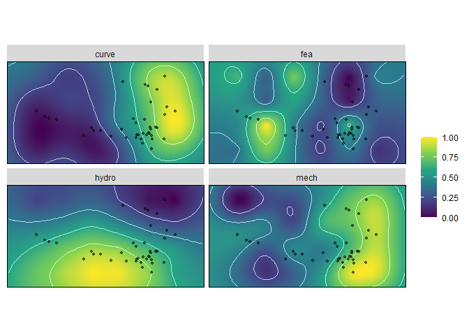
To calculate adaptive landscapes based on groupings, first a population of landscapes is generated using generate_weights() and calc_all_lscps():
weights <- generate_weights(n = 10, data = kr_surf)
all_landscapes <- calc_all_lscps(kr_surf, grid_weights = weights)
all_landscapes
#> An all_lscps object
#> - functional characteristics:
#> hydro, curve, mech, fea
#> - number of landscapes:
#> 286
#> - weights incremented by:
#> 0.1
#> - new data:
#> 40 rowsOptimal landscapes for groups are then calculated using calcWprimeBy() and can be statistically compared using multi.lands.grp.test():
wprime_by_Group <- calcWprimeBy(all_landscapes, by = ~Ecology)

wprime_by_Group
#> - Ecology == "M"
#>
#> Optimal weights:
#> Weight SE SD Min. Max.
#> hydro 0.15 0.06455 0.1291 0.0 0.3
#> curve 0.00 0.00000 0.0000 0.0 0.0
#> mech 0.00 0.00000 0.0000 0.0 0.0
#> fea 0.85 0.06455 0.1291 0.7 1.0
#>
#> Average fitness value at optimal weights:
#> Value SE SD Min. Max.
#> Z 0.7686 0.01039 0.02078 0.7444 0.7927
#> -----------------------------------------
#> - Ecology == "S"
#>
#> Optimal weights:
#> Weight SE SD Min. Max.
#> hydro 0.85556 0.02422 0.07265 0.8 1.0
#> curve 0.05556 0.02422 0.07265 0.0 0.2
#> mech 0.05556 0.02422 0.07265 0.0 0.2
#> fea 0.03333 0.01667 0.05000 0.0 0.1
#>
#> Average fitness value at optimal weights:
#> Value SE SD Min. Max.
#> Z 0.7496 0.005665 0.017 0.7326 0.7835
#> -----------------------------------------
#> - Ecology == "T"
#>
#> Optimal weights:
#> Weight SE SD Min. Max.
#> hydro 0.00 0.00000 0.0000 0.0 0.0
#> curve 0.85 0.06455 0.1291 0.7 1.0
#> mech 0.15 0.06455 0.1291 0.0 0.3
#> fea 0.00 0.00000 0.0000 0.0 0.0
#>
#> Average fitness value at optimal weights:
#> Value SE SD Min. Max.
#> Z 0.7646 0.008862 0.01772 0.744 0.7852
#>
#> - method: chi-squared, quantile = 0.05
summary(wprime_by_Group)#> Optimal weights by Ecology:
#> W_hydro W_curve W_mech W_fea Z
#> M 0.15000 0.00000 0.00000 0.85000 0.76856
#> S 0.85556 0.05556 0.05556 0.03333 0.74959
#> T 0.00000 0.85000 0.15000 0.00000 0.76457
plot(wprime_by_Group, ncol = 2)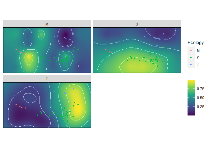
tests <- multi.lands.grp.test(wprime_by_Group)
tests
#> Pairwise landscape group tests
#> - method: chi-squared | quantile: 0.05
#>
#> Results:
#> M S T
#> M - 0 0
#> S 0 - 0
#> T 0 0 -
#> (lower triangle: p-values | upper triangle: number of matches)To cite Morphoscape, please run citation("Morphoscape").