Compute optimally weighted adaptive landscapes

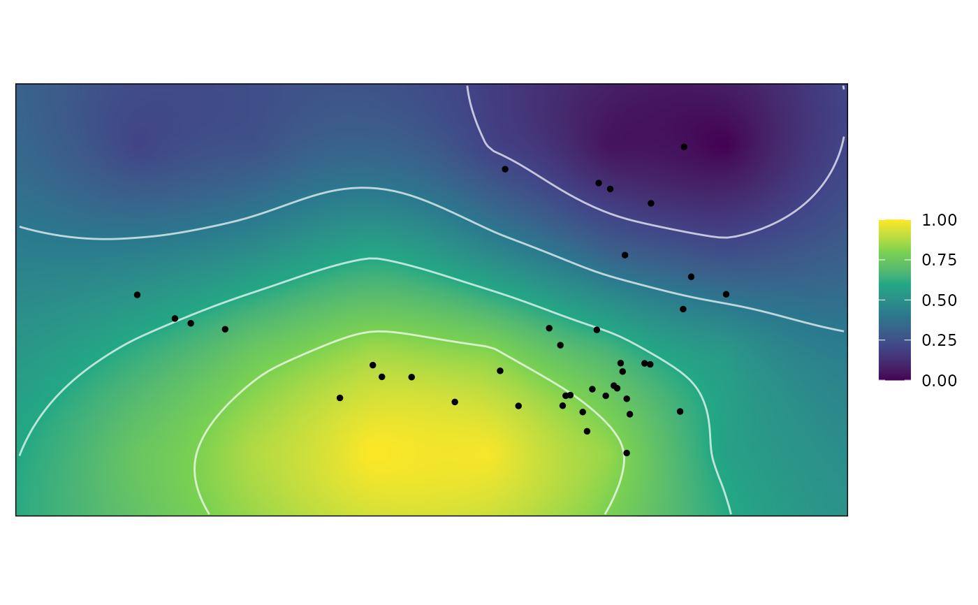
calcGrpWprime() computes the optimally weighted adaptive landscape by searching through the adaptive landscapes formed from sets of weights and performance surfaces, and finding the set of weights that yields the greatest overall (average) fitness value (Z) across a sample of data or a subset thereof.

Usage

calcGrpWprime(x, index, method = "chi-squared",
              quantile = 0.05)
# S3 method for grp_Wprime
print(x, 
      digits = max(3L, getOption("digits") - 3L), ...)

Arguments

x

for calcGrpWprime(), an all_lscps object; the output of a call to calc_all_lscps.

for print(), a grp_Wprime object; the output of a call to calcGrpWprime()

index

an optional vector of indices indicating which subset of the new_data dataset originally supplied to krige_surf should be calculated. Can be specified as a vector of numerical indicies, logical indices, or row names. If unspecified, the optimal weights will be computed using the full sample. Supplied to subset, so the name of the dataset containing the subsetting variable does not need to be included if the subsetting variable is in new_data. See Examples.

method

the method used to compute the optimal weights. Allowable options include "chi-square" (the default), "quantile", or "max". "chi-square" and "quantile" involve averaging across the best several sets of weights, whereas "max" uses the singular best set of weights. Abbreviations allowed. See Details.

quantile

when method is "chi-square" or "quantile", the top quantile used to determine the best sets of weights to be included in the average to compute the optimal set of weights. Should be a number between 0 and 1, with a low value indicating that only the few top sets of weights will be used. Ignored when method = "max".

digits

the number of significant digits to print.

...

passed to print.default.

Details

calcGrpWprime() calculates an overall fitness score for each set of weights based on the average weighted fitness values of the indexed subgroup. The set of weights that optimizes this score is then produced as the weights defining the optimal adaptive landscape for that subgroup. The way the final set of weights is computed depends on the argument to method. When method = "max", the single best set of weights is used. However, often many of the upper sets of weights perform equally or nearly equally as well as the best set. It is instead recommended to use "quantile" or "chi-squared" methods. When method = "quantile", the top $X\%$ of weights are averaged to compute the optimal weights, where $X$ corresponds to the value supplied to quantile. When method = "chi-square", the chi-squared value $\chi^2_i$ is computed for each set of weights $i$ as $$\chi^2_i = -2 \log \frac{Z_{max}}{Z_i}$$ where $Z_{max}$ is the largest $Z$ among the weights, and a p-value is computed for each $\chi^2_i$ value using a $\chi^2$ distribution with 2 d.f.; any set of weights with a p-value less than quantile is included to be averaged to compute the optimal set of weights.

Value

A grp_Wprime object, which contains the following components:

Zprime: a list containing the optimal weights and the Z value they yield (wn), and, if method is "chi-square" or "quantile", summary statistics about the best sets of weights used to compute the optimal weights, including the standard error (wn.se), standard deviation (wn.sd), and range (wn.range).
W: a matrix containing all sets of weights (i.e., those supplied to the grid_weights argument of calc_all_lscps()) along with the Z value each yields, ordered in descending order by the yielded Z value. When index is specified, the resulting Z values are computed only using the indexed subset.
Wprime: a wtd_lscp object containing the optimal weights (W) and the landscape grid and sample functional characteristcs weighted by the optimal weights.

References

Dickson, B. V., Clack, J. A., Smithson, T. R., & Pierce, S. E. (2021). Functional adaptive landscapes predict terrestrial capacity at the origin of limbs. Nature, 589(7841), 242-245.

Jones, K. E., Dickson, B. V., Angielczyk, K. D., & Pierce, S. E. (2021). Adaptive landscapes challenge the "lateral-to-sagittal"" paradigm for mammalian vertebral evolution. Current Biology, 31(9), 1883-1892.

Examples

data("warps")
data("turtles")

warps_fnc <- as_fnc_df(warps, 
                       func.names = c("hydro", "fea"))

kr_surf <- krige_surf(warps_fnc, new_data = turtles)
#> [using ordinary kriging]
#> [using ordinary kriging]
#> [using ordinary kriging]
#> [using ordinary kriging]

grid_weights <- generate_weights(n = 3, data = kr_surf)
#> 4 rows generated

all_lscps <- calc_all_lscps(kr_surf,
                            grid_weights = grid_weights)
                            
wprime_S <- calcGrpWprime(all_lscps,
                          index = Ecology == "S")
wprime_S
#> Optimal weights:
#>       Weight SE SD Min. Max.
#> hydro      1 NA NA    1    1
#> fea        0 NA NA    0    0
#> 
#> Average fitness value at optimal weights:
#>    Value SE SD   Min.   Max.
#> Z 0.7835 NA NA 0.7835 0.7835
#> 
#> - method: chi-squared, quantile = 0.05
plot(wprime_S)